This project started back in April 2021. I just had finished my first undergrad controls class, UC Berkeley's ME 132, and I was aching to get some hands-on experience. You see, I had taken this course during the pandemic, so I had no chance to implement any of the wonderful control strategies we had learned about. At the time, I was also a part of a Human-Robotics Interaction Research Group, "Metrobot", which had just received a $10,000 grant to build some cool robots. After experimenting with standard wheeled chassis robot driveframe designs, I convinced my team to move forward with a balancing, wheeled robotic platform instead. And thus, the idea for Chickenbot hatched.
The first question I usually get when talking through Chickenbot is: "Why does it have only two legs and two wheels? Wouldn't it fall over?". The answer to that is, well, yes, while this robot design requres complex control systems, it seeks to address the shortcomings of other common robotic drivetrains. Many traditional robotic drivetrains designs are limited in mobility. Wheeled robots are incapable of agile movement, while legged robots are inefficient and require intensive control theories. I became curious about hybrid robotic locomotion strategies; a wheeled, legged robot. In theory, robots of this nature could provide many of the advantages of a legged robot and a wheeled robot. If the wheels do not turn, then they function as static feet. When on flat terrain, however, the wheels are allowed to rotate to stabilize the robot like an inverted pendulum. This robot does not have sufficient degrees of freedom to walk on it's wheels as feet, but such an idea would be worth exploring in future designs.
Chicken Bot got its' name from original concept sketches, which looked mildly like the side profile of a chicken. The project was initially funded through a grant by UC Berkeley's Student Technology Fund, as a human-robotics interaction research project. The robot was designed as a platform to conduct various experiments, from applications such as intents classification to measuring emotional response. The current objective for the robot is to teach it to autonomously play fetch.
Many of the key mechanical features for this robot were inspired by the Ascento robot, which started as a research project at ETH Zurich. This robot aims to build off of their work, expanding capability to feature a multipurpose robotic arm as well.
The Chicken Robot is designed to function as a simple inverted pendulum. Each of its' legs is a separate four-bar linkage mechanism, allowing for motion along a prescribed path with one degree of freedom. The head and manipulator mechanism (not pictured) has an additional two degrees of freedom, allowing the robot's camera suite to track an object passing overhead.
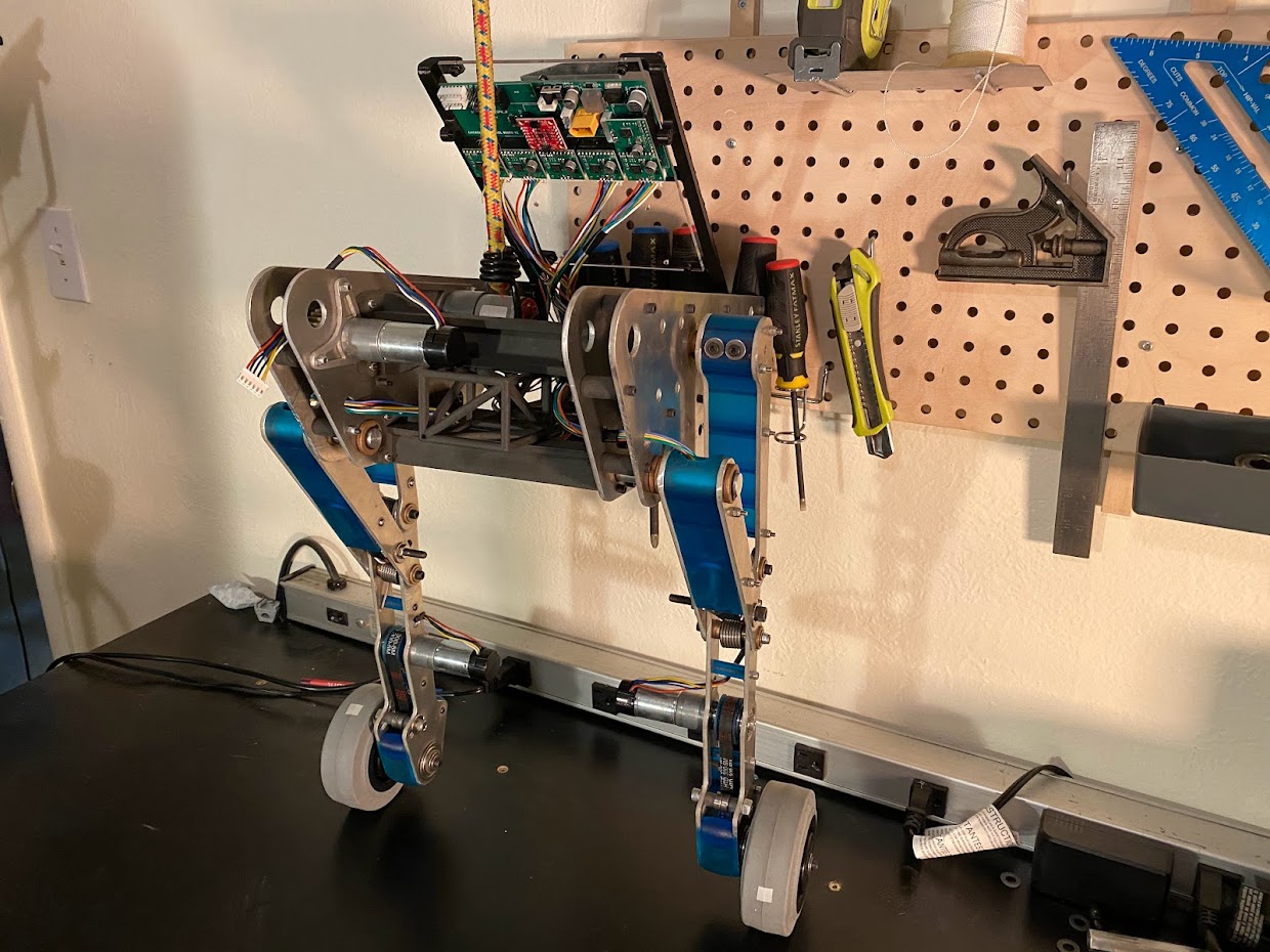
The chicken robot is designed for compact mechanical integration, accessible electrical components, and easily serviceable wear components. The robot stands around two feet tall up to its' shoulder, and features a custom printed circuit board, hybrid 3D printed / laser-cut aluminum chassis, and a NVidia Jetson Nano processor onboard, equipped for machine learning. The robot also features a series of Intel Realsense Cameras, enabling depth perception and precise location tracking.
I modeled the four-bar linkage of the legs in Desmos, a simple online graphing calculator, to determine the path they would take through the leg's range of movement. Here's what that looks like:
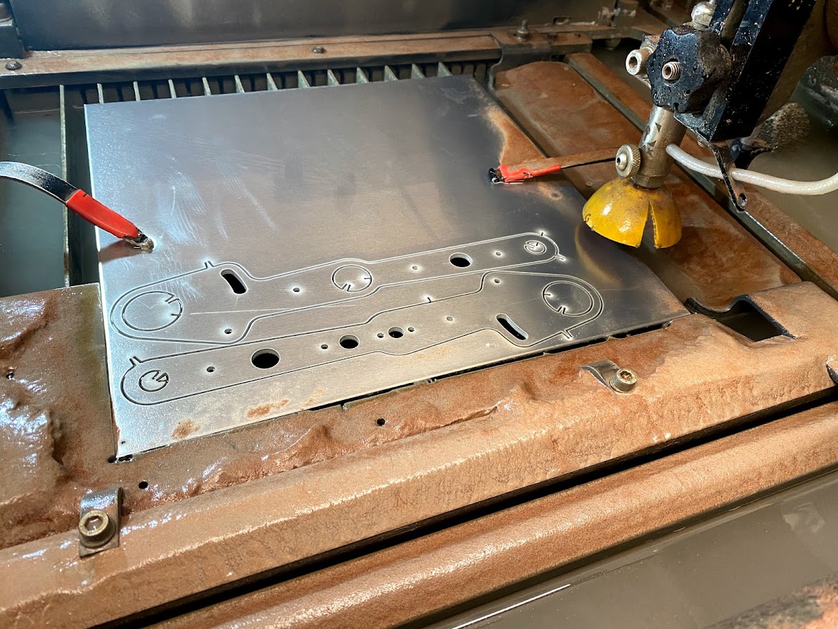
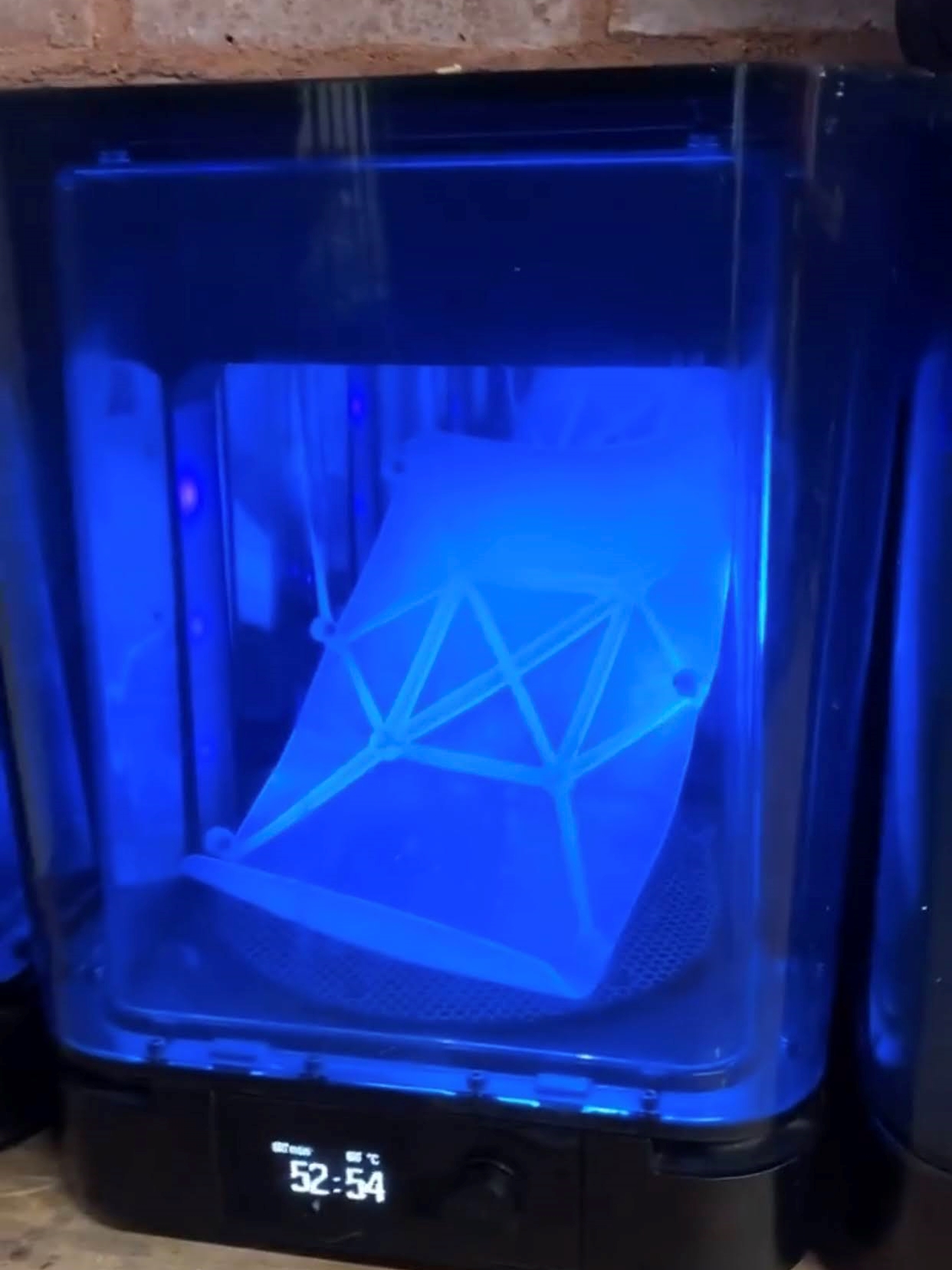
I manufactured the majority of the parts in Formlabs' machine shop when I was working there in Summer '21. Most of the parts were either cut our of aluminum on a waterjet or 3D printed via SLS or SLA technologies, but some parts were also manually milled and turned.
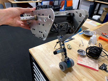
One of the greatest perks of digital fabrication is the speed at which you're able to progress through various designs. I began assembling the robot shortly after finishing the main chassis design, and before I knew it, it was mechanically ready to roll.
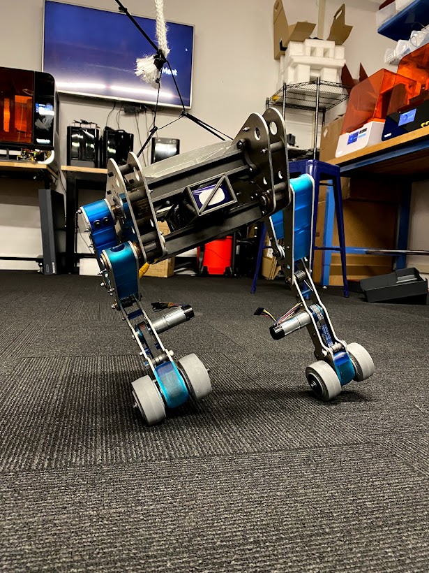
Finally, I had all of the parts completed, and I assembled them all together into a finished robot:
In August-December 2021, a new team of people joined me to help improve the still-nameless and still-headless Chickenbot. One collaborator, Kai Chorazewicz, helped massively by designing a custom printed circuit board to incorporate all of the electrical components needed to bring this robot to life. Chickenbot is equipped with an ESP32 microcontroller which collects data from the various sensors onboard, as well as controls the comanded motor actions. Chickenbot's PCB v2 con control and monitor six DC motors with encoders (capable of current feedback on four), two Servo motors, and a 12-DOF inertial measurement unit (IMU). Chickenbot can also connect with a host computer over bluetooth, an external high-level control board over UART-Serial, and over the internet as well, although IOT-Chickenbot capabilities would likely be handled over the high-level control board and are as of yet unimplemented.
Balancing an inverted pendulum robot is an issue which has been tackled countless times in academia, so I must say that I was surprised how many issues I ran into when implementing the preliminary control systems. I started off with a state-space approach for balancing the robot, using four states. The state space controller would provide full state control of the robot's vertical angle, pitch angular velocity, left-right turning (yaw) angular velocity, and overall forward-backward wheel velocity, to start.
However, I faced tons of issues getting a state space controller to adequately stabilize the robot. I have not fully explored the capabilities of a modern state-space control strategy, but after several months of work, I shelved the idea and began with the simplest approach: PID.
I first tried one simple PID loop, which calculated the robot's pitch angle using the gyro alone, and commanded it to take on an angle that I measured when the robot was near-balanced. I quickly learned that measuring an absolute position from angular velocity alone had many drawbacks, and then implemented a complementary filter to correct the robot's state estimation using the accelerometer's gravitational reading to eliminate steady-state drift. The robot could then utilize the high frequency response of the IMU and the low frequency response of the accelerometer in order to more accurately synthesize the two into a more consistent final reading.
Once I had a more accurate state estimator, I began to see success in the introductory controls schema. In other words, chickenbot had her first steps on training wheels:
At this point, Chickenbot still needed a safety apparatus to stand on her own, but after several hours of tuning, she was ready to venture out into the real world:
The robot's first balancing was achieved on May 20th, 2022.
Unfortunately, this control strategy with a single PID lop still leaves a lot to be desired. Firstly and most importantly, the robot cannot be controlled: with the current strategy, the robot sends a motor output to control the robot's pitch angle alone. To fix these shortcomings, I did more research into successful PID balancing strategies, and found a wonderful project by Shay Sackett which seemed to provide exactly what I was looking for. I added a second nested PID loop to control velocity at the same time as the robot's angle. With this, and a third PID loop to control the differential motor output sent to the left and right wheels to permit yaw control, we finally began to see some results:
After adding the neck, which changes the robot's center of gravity, the new control strategy was unfortunately no longer robust in keeping the chassis balanced. New control strategies are in the works which implement a third nested PID loop to control the robot's commanded tilt angle based on measurements of the robot's current angle as well as the angular velocity of the robot. Ideally, this should allow the robot to find the angle at which it is balanced, and the tilt's derivative with respect to time is zero. Then, the controller commands the wheels to meet a desired velocity on top of what is required to keep the robot balancing. I will update this section to provide more detail about the control strategies once I successfully work out all of the kinks.
The goal of this project is to teach a wheeled, legged dynamically stabilizing robot how to play fetch, as an exercise in human-robotics interaction. More specifically, the goal is to throw a standard tennis ball and have the robot determine where the ball lands, and then retrieve it and bring it back to a desired position. To do this, we have designed and built a head and grasper for the existing robot chassis, and incorporated computer vision systems to allow the robot to perceive its surroundings and precisely navigate through the world. The scope of the project which will be evaluated for this class is not the entire robot, as much of the robot's development occurred prior to this class. Rather, we will be focusing on applying the concepts from class to make the robot perform tasks using ROS. We will design and build a grasper mechanism for the robot, and implement computer vision to allow the robot to autonomously navigate to waypoints in space.
The overall, long-term objective of the project is for the chicken robot to play fetch; using a suite of sensors, the robot will eventually track the location of a tennis ball, move to where the ball is located, grasp it, and then return the ball to the sender. Unfortunately, we did not have time to implement all of these goals due to unforeseen mechanical issues requiring an extensive chassis redeisgn, but we made sufficient progress with the areas of this project which relate to the curriculum of EE 106A. This project is interesting because the field of Human-Robotics Interaction is nascent, and massively growing. Countless opportunities arise from the interaction between humans and robots, but there are many shortcomings in traditional robotic systems, such as wheeled and legged robots. Wheeled robots allow for simple actuation and control architectures, but can only traverse a limited set of environments. In contrast, legged robots can traverse a variety of terrains, but require complex planning and control strategies in order to be successful.The objective for this robot was to aim for a hybrid between the two - a legged, wheeled robot, to take advantage of the efficient and simple locomotion offered by wheels, while still reaping the rewards of versatility offered by legs.
The primary objective of the contributions for this class are limited in scope to a subset of the work displayed on this page. For the final project of EE/ME 106A, the deliverables in-scope are as follows. We have designed and implemented a 3-DOF manipulator and grasper for the chicken robot, set up ROS functionality on a Jetson Nano processor from scratch, and implemented vision systems to detect the location of a standard tennis ball relative to the robot. Further, we have implemented a custom serial communication protocol to permit information transfer between the embedded control board and the higher-level vision strategy board with ROS connecivity, and we are able to track the robot's location precisely in space using pre-built V-SLAM techniques included with the tracking camera used in this project. To do this, we overcame interesting obstacles in every step of the process, from mechanical failures and redesigns to electrical replacements, fried motors, broken gearboxes, ROS install nightmares, and everything in between. Real-world applications of this project are numerous, an agile robotics platform designed for human-robotics interaction could have applications in automation, customer service, disability assistance, medicine, delivery, and more.
This phase of the project begins to utilize the electronic equipment originally purchased several years ago, before anyone had any idea what to do with the components. Chickenbot takes advantage of the following hardware:
In addition to the components listed above, the mechanical aspect of this project utilizes the actuators below:
Notably, we experienced many issues with Pololu brushed metal gearmotors. So far in this project, over five of this type of motor have failed, and it is time to redesign away from these expensive and improperly sized actuators.
This robot features a compliant grasper with three degrees of freedom which doubles as Chickenbot's head. It also houses the vision sensors described in the previous section. The manipulator meets many design creiteria set forth for maximal versatility and utility.
The robot's manipulator must...
To achieve these criteria, a compliant grasper design was chosen on a two-DOF arm. A compliant grasper offers many benefits over the common rigid graspers often included in robotics projects. Firstly, compliant parts are inherently far safer than rigid components, especially when in a location that pinches tightly together, and is the main point of interaction between the robot and a human. A compliant grasper reduces the risk of human injury in HRI use. Secondly, a compliant grasper is oftentimes more versatile than a rigid grasper, as it can conform to form a more complete hold on objects with eccentric shapes. As an example, see how the robot's grasper deforms to hold a ball in place tightly.


The geometry of the grasper utilizes the fin ray effect, and the current grasper is the sixth iteration of this component. There is certainly still room for improvement for the rigidity of this manipulator, as well as the overall fit and finish, but it is adequate in meeting the requirements of this project, so shortcomings will be addressed further in the future. Current shortcomings of the grasper are that it is not rigid enough in out-of-plane directions, such that the graspers rotate inward if carrying a load heavier than the tennis ball it was designed for. This could be solved by making the extrusion pattern thicker in the vertical direction, as well as increasing the rib thickness of the compliant links.
The actuator is powered by the MG-996R Servo Motor, which offers a wider rotational range than is needed for this application, at 180 degrees. The strength of this motor is also adequate in supplying the necessary forces to manipulate a 0.5kg payload. The two halves of the beak mechanism are coupled together using a standard set of partial spur gears, which are mechanically incapable of overactuating. The motor's placement on this articulated link is such that it is as close as possible to the pivot point, such that the manipulator is agile and does not require any more energy to move than is needed.
Next we will consider the mechanical design of the neck and head subsystems. For context, see the included diagram of a cross section of the neck manipulator, which we will explain in detail below.

The manipulator is composed of two rigid links, the lower link being the neck and the upper link being the head. The head is able to nod up and down, as is the neck system as a whole. The head's tilt system is actuated by a DS-3235 Servo Motor, which is located as close to the parent joint as possible to minimize the link's moment of inertia. The torque output of this motor is transmitted to the endpoint linkage by a belt and pulley system, which is tensionable to ensure near-zero backlash and precise locational control. The belt tensioning system is custom and converts the belt's tension into tensile loading of a pair of standard bolts, so that there is little risk of the belts becoming untensioned during standard operation. This is an improvement over positive-style belt tensionining mechanisms, such as those utilizing cams. The lower neck joint is rigidly coupled to a dead-axle design which is driven by a Pololu metal gearmotor with a 227:1 reduction using standard spur gears. Unfortunately, the gearmotors selected for this application were drastically underpowered compared to what was required. When the motors were purchased, the grant was on the verge of expiring, so the design progressed forward without the proper calculations being verified, and as it turns out, more powerful motors are required. The result is that the motors tend to burn up rather quickly if allowed to operate at full current for longer than a second or two, turning Chickenbot into a Fried Chickenbot.
We established UART communication between the ESP32 and JetsonNano. The ESP32 sends sensor information to the Jetson Nano, which then sends the information to a ROS Topic called “nano_interface”. As for the other direction, the JetsonNano sends commands to the ESP32 to actuate the chickenbot.
The sensor information includes 13 data points: the chickenbot’s three acceleration measurements (x, y, z), three orientation measurements (x, y, z), two wheel speeds (left and right), two hip angles (left and right), neck angle, head angle, and grasper angle. We chose to send most of the values as floats, which occupy 4 bits, to store very accurate information, but we set a few variables as integers, which occupy 2 bits, and chars, which occupy 1 bit, since they need less specificity.
On the ESP32 side, we created a union data type, called sentPacket, to store the sensor data. All variables in a union point to the same memory location. The union contains a structure and a character byte array. When we created sentPacket instances, we assigned values to the structure in the instance. We then directly write the sentPacket instance (which is automatically converted into binary data with the Serial.write function in C++) from the ESP32 to the Jetson Nano. We used the newline symbol, “\n”, appearing twice in a row to indicate the end of a message. This also took up 1 bit. Our explanation for why we use “\n” twice is below.
We discovered that the data was chunked into 4 bits at a time in the union. For example, with just a character in the union, the character occupies one bit and the union will zero pad the remaining input, which means fill the remaining bits with 0’s. A float, which conventionally occupies four bits, will not require zero padding.
On the Jetson Nano side, we read incoming messages in the serial port, one bit at a time, and we used the struct library in Python to unpack the bit values into Python variables. We checked for the “\n” symbol appearing twice consecutively to determine when we received a complete message. We then stored all of these values into a ROS message and published the message to a topic called “sensor_data”.
Sometimes, the grasper angle was sent to a numerical value with the ASCII equivalent as “\n” because we stored the grasper angle as a character. Initially, when we only used one newline symbol to indicate the message’s end, this cut our messages short. That’s why we use two consecutive newline symbols for the message’s end.
The command information sent to the low-level control board includes eight values: two "character" type state positions, and several "float" state commands: the neck's position, forward wheel velocity, angular turning velocity, commanded angular velocity of head motor, commanded hip angle for leg height, and the velocity of the grasper servo. All of the data types are neatly packaged into a struct, and then into a union which is also accessible as a byteArray in C++.
On the Jetson Nano, a ROS Topic called “controller_commands” takes the command information as a message. For any messages published to “controller_commands”, the communication node packs the message’s variables into the appropriate bit values using the struct library, and is written to the serial port.
To fetch the ball, we first need to locate where the ball is in both D435i frame and world frame, i.e. getting D435ipD435i,B and WpWB. This can be divided into three tasks:
1.) Determine the position and orientation of D435i RGB-D camera in world frame gW,D435i
2.) Determine the ball’s position D435ipD435i,B in D435i frame.
3.) Transform from D435i frame to world frame WpWB = gW,D435iD435ipD435i,B
The first task can be done using T265 tracking camera’s position and orientation output and a constant transformation matrix between the two cams.To do the second task in a computationally efficient manner, we choose to use RGB and depth images instead of the point cloud generated by D435i. Firstly, we use openCV to detect the ball in 2D[1]. As shown in the figure below, we first convert the RGB image to HSV color(bottom right image) for more robust color thresholding. We then threshold the ball and remove noise by eroding small objects and dilating big objects in the binary threshold result(top right image shows the effect after noise removal). Next, we find the biggest outmost contour and calculate the ball center and area using the moments of the contour(bottom left image).

Secondly, we go from 2D pixel coordinate [u,v]T to 3D D435i coordinate[x,y,z]T , we use the depth value z from depth image, and the camera calibration matrix K.

When going from 2D to 3D, as shown in the figure below, we utilize the pixel coordinate and depth of a small patch of points around the center of the ball instead of just a single point at the center because depth value may not be available at a single point due to uncontrollable noises. We average the 3D D435i coordinates of the patch points to get the surface position vector psurface and increment it by the radius vector rball to get the real ball position. This is critical if we want the robot to grasp the ball since the tennis ball we use has a radius of as large as 3.25cm.

When the ball is moving fast, chances are that the detection can fail some time. We need to tell the robot where to look for the ball so that the ball does not get lost forever. That’s why we implement the ball prediction algorithm. We have four prediction modes:
1.) Static: ball stays in the same place
2.) Uniform Velocity: ball moves at the last estimated velocity
3.) Decaying Velocity: ball’s velocity decays exponentially vk+1 = αvk (α<1)
4.) Dynamic: take into account both gravity and bouncing off ground.
All predictions are made in world frame. We finally used the Decaying Velocity mode because of the limited frame rate we can achieve on JetsonNano, but we initially implemented the Dynamic mode because we hoped that we can throw the ball and let the robot play fetch. The following video shows how well the Dynamic mode can predict the ball trajectory if we have enough frame rate(60Hz achieved on Lenovo Y7000P). The reason why we need a high frame rate is that we have to capture an accurate initial velocity at lost time to perform accurate dynamic prediction when the velocity is changing fast. Missing even 0.1s can lead to significant error.

In the above video, the moving object is the ball. The red vector originating from the ball shows the direction and magnitude of the estimated velocity. When the detection is not lost during the initial upward motion, a red ball point cloud will be visualized. Halfway through the upward motion, when the ball coincides with the red axis, the ball moves outside the camera's horizon and detection is lost. The ball point cloud stucks there, but the estimation of ball position and velocity continues using prediction. We can see the ball follows a parabola trajectory, and bounces up when hitting the estimated ground.
Here’s how the Dynamic mode predicts the ball position and velocity. When the ball is still in the air, the position and velocity in the world xyz direction(world xy are always horizontal and world z is always vertical) are predicted as follows:

To determine whether the ball will hit the ground during the t ∈ [0, Δt] period, we solve the following equation for thit. The ground height zgnd can be obtained either by forward kinematics from camera to wheel, or by initializing the world frame properly so we know in advance the ground z coordinate in the world frame:
pz,k+vz,kthit-1/2gthit2=zgnd
If thit < Δt, then the ball will bounce up at z velocity vz,up = -avz,hit where a = 0.7 is obtained by observation.
We also predict whether the ball will bounce up again by comparing the time between the first and second bouncing up Δtbounce = 2vz,up / g and the remaining time after the first bounce tremain = Δt - thit. If the ball will bounce up again, it means that vz,up is small enough to be neglected without hurting the ball-refinding purpose of prediction, and we will directly predict vz,up = 0 for simplicity.
Now that we have knowledge of where the ball is and where to look for the ball when lost, we need to control the robot to stare at the ball by facing the camera towards the ball, and drive to the ball to fetch it. By mechanical design, when the camera is facing towards the ball, so is the robot.
All of these can be done using the same feed-forward + P velocity control framework. Suppose we want any time-variant state x(t) to track a time-variant reference xd(t), and we know we can directly command the motors to follow a specific rate of change on the state dx/dt. We first design the desired error dynamics as an exponential decay, where kp is some positive value.
d(xd-x)/dt=-kp(xd-x)
Then, we reformulate this to the control law on dx/dt:
dx/dt=dxd/dt+kp(xd-x)
Intuitively speaking, the rate of the actual state dx/dt should always exceed the rate of the desired state dxd/dt (feed-forward) by a proportional amount of error kp(xd - x)(P control) in order for the error to decay exponentially.
How does this apply to our controls? As is shown in the figure below, we have control over the head motor pitch rate dϕ/dt, the yaw rate dψ/dt generated by wheel differential velocity, and the forward velocity dp/dt generated by wheel average velocity. The former two are used for staring control and the latter two are used for drive-to-ball control. There’s no conflict in controlling the yaw rate since the goal for yaw in both controls are facing towards the ball.
In pitch rate control(left figure), the goal is to let the camera center line coincide with the ball vector. The pitch rate we control is defined to be the angular velocity dϕ/dt of D435i with respect to the neck since that’s what the head motor is doing. Instead of defining absolute pitch values for D435i and the ball vector, we only need to define their difference(pitch error) ϕd - ϕ, which can be easily measured in D435i frame.
Similarly, in yaw rate control, we define the yaw rate dψ/dt as the z angular velocity of the robot with respect to world, and the yaw error ψd - ψ as the yaw difference between the ball vector and the D435i center line.
In forward velocity control, we define dp/dt as the forward velocity of the center of wheel with respect to the world, and the position error pd - p as the horizontal distance to the ball, minus the distance we want the robot to keep from the ball.

Before we can do the control, we also need estimates for the rate of change of the desired states dϕd/dt, dψd/dt, dpd/dt is just the ball velocity with respect to the world, so we just need to find the former two desired angular velocities. Since we already have plenty of estimation of linear velocities and positions, we calculate the angular velocity by dividing some linear velocity by some radius. As shown in the figure below, we define the plane formulated by the pitch axis and pball as Pitch Plane, and the plane formulated by the vertical axis passing through D435i center and pball as Yaw Plane. For simplicity, we denote pball := pD435i,B. We denote the component of pball orthogonal to the rotation axis as pball,⊥. It will be the “radius” we use to calculate angular velocity. We then calculate the linear velocity difference between the ball and the center of D435i vdiff = vball - vD435i. vdiff can be decomposed to vdiff,⊥ that is orthogonal to the Yaw or Pitch Plane, vdiff,∥,∥ that is parallel both to the Yaw or Pitch Plane and to pball,⊥, and vdiff,∥,⊥ that is parallel to the Yaw or Pitch Plane, and orthogonal to pball,⊥. vdiff,⊥ will be the “linear velocity” we use to calculate angular velocity. We see that the angular velocity for both pitch and yaw can be expressed in the form of ω = vdiff,⊥ / pball,⊥. In vector form,

Where the Aligned D435i Frame is originated at the center of D435i, with its x axis pointing horizontally forward and z axis pointing vertically upward. But calculating orthogonal components is a bit tricky. Fortunately, we noticed that we can change orthogonal component calculation to simply extracting the xyz components using geometric properties. In particular, for pitch rate calculation in the left figure,

since pball,⊥ cross produced with vdiff,∥,∥ and vdiff,∥,⊥ won’t point in x direction. Moreover, pball,⊥ = pball,yz for pitch rate calculation. Same methodology also applies to yaw rate calculation. Thus, we now have a much simpler calculation where all vectors are readily available.


In the next section, you will see a video of the control performance of the head motor pitch control. We can see that the controller keeps the ball reliably in the center of the image, and with further tuning could do so with an even faster settling time.
Numerous other design considerations were taken into account when designing the head manipulator. Inspiration was drawn from biological sources wherever possible, resulting in geometry which resembles ball-and-socket joints, for their high actuation bounds. The neck is capable of lowering to pick an item up off the ground while the robot is balancing, or to stow on the robot's back in a compact orientation. See the renders of the final robot in verious configurations below:


Below is a video of the ball tracking live on the Jetson Nano. Unfortunately, the power electronics responsible for powering the 5V source that the Nano needs are not capable of sustaining the power draw of the nano due to an undersized buck converter, which can only handle 2A instead of the 4A that the Nano requires during heavy computation. As a result, we were unable to show what some consider to be the most important functionality that chickenbot has. Chickenbot is equipped with a 2.5W, 4Ohm Speaker and power amplifier, for the sole purpose of making assorted clucking noises during operation. When the robot grabs a tennis ball with the Jetson Nano running without computer vision running, it will make the noises that you would expect from a friendly household chicken. We have further plans to implement a variety of different tonalities in the audio files that Chickenbot plays, perhaps to communicate different emotions.
Overall, while our group was not able to play fetch with Chickenbot as we had initially hoped to, we are stil satisfied with the functionality that we accomplished. While it would have been wonderful to have the robot balancing and driving around the lab on its own, unfortunately the proven balancing functionality from before the start of this course failed to work correctly after the addition of the neck and arm manipulator. A more extensive rework of low level controls architecture is underway, and the work we have done here is prepared for implementation as soon as the robot is able to reliably be controlled with a changing center of mass. As far as the communication architecture is concerned, we have verified that the Jetson Nano is able to send velocity commands to Chickenbot and direct it toward the ball. As a result, further work is only blocked by the aformentioned improvements to the foundational electrical, hardware, and controls strategies, which were outside the scope of this course anyway.
This project has had many contributors over the two years since it first began, but in the scope of ME/EE 106A, the team is as follows:
Michael is an undergraduate student who has officially, as of submitting this assignment, graduated from UC Berkeley with dual degrees in Mechanical Engineering and Business Administration. He has been building robots since 2015, and has loved engineering for as long as he can remember. After graduating, he has accepted a position in a stealth mode research facility in the bay area. For more information, see my about page.
Hanwen Wang is an MEng student majoring in Mechanical Engineering: Control of Robotics and Autonomous Systems. In this project, he is mainly responsible for the openCV ball detection, ball prediction, and the staring and drive-to-ball control algorithms.
Carolyn is a junior studying applied mathematics and computer science. In this project, she worked on serial communication. A fun fact about her is that her favorite animals are ducks, though chickens are neat too!
Although it feels like this project has experienced nearly every issue imaginable, it has been an outright pleasure to learn from the chaos that is the integration of discretely developed electromechanical systems. This project went through countless nightmares in its' development. Despite failures of three motors, battery concerns, and worries at having accidentally fried both Michael's Laptop as well as the Jetson nano (everything was okay, thankfully), we successfully managed to actuate the head to track the tennis ball’s pitch angle with zero steady state error and a fast response time. Since pitch, yaw, and forward movement all use the same feedforward + proportional control strategy, we believe that our one succesful implementation may serve as validation for all of them, and the chicken robot has the potential to drive itself to the ball as long as the battery and mechanical subsystems are working well.
The ball detection and prediction algorithms on which the control algorithms are based also worked well. We did block-wise validation for all of them and end-to-end test in the above control test, and results are positive.
The soft graspers on the head can also grasp a tennis ball firmly, and we’ve also validated the serial communication between JetsonNano and ESP32 by letting the chicken cluck when it performs grasping. The speaker controlled by JetsonNano can receive the grasping signal from ESP32.
For balancing, we are currently implementing a new strategy, but did not have adequate time to finish tuning the necessary control constants to a successful operating range.
In terms of difficulty, this project was a lot to bite off. With the power electronics we used, our motors can only be velocity controlled, making most torque control strategies infeasible. Unfortunately, this prevented us from successfully implementing a strategy based on the lagrangian method of calculating the system's dynamics. As a result, our poor motor control only increases the difficulty of balancing with an already highly nonlinear rboot, with a changing center of mass and inconsistent ground friction. The limited computational power of uor JetsonNano also limited the frequency our algorithm can run, which makes highly dynamical tasks such as tracking a ball that’s thrown by the user very difficult. However, we haveshown that on a more powerful computer, the computer vision algorithms developed work quite quickly.
Initially, we wanted to import the robot's CAD model into a URDF so that we could visualize and better control the robot's motion with a user interface. Unforunately, we learned that due to a URDFs' tree structure, they do not support four-bar linkages, as a single link would have more than one parent link. On top of this, our battery is poor quality, motors are easy to fry, and there is too much play and mechanical friction in the leg manipulators. So much chaos!
If we had additional time, we would first improve the hardware: replacing the motors with brushless torque-controllable ones, and upgrading the battery. Then, we would prioritize integrating the balancing, ball staring, and drive-to-ball control strategies to create a solid foundation. After the robot can stand on its own feet and follow us, we will proceed for automatic grasping. Rest assured that the eventual final product will be documented in a future youtube video, and will be made available right here on this website!
While this robot is still in development, it has been a wonderful platform for diving deeper into the field of control systems and robotics. We have combined our collective knowledge from over ten years building robots, and despite this, we all learned more and more each day. I believe this robotics platform has high potential for other spaces where robots are expected to work alongside humans. Building on this idea, the long-term objective of this project is to create a human-scale, ostrich sized robot with a multi-axis manipulator. This robot could assist human workers or take over many simple tasks. This system is still a long ways out, but paves the road forward for an exciting future of collaboration between humans and robots.
All code for this project is available at our github repository: https://github.com/metrobot-research/embedded/tree/SerialRewrite
Thank you for reading, and I hope that you enjoyed following along!